SRNCA blogpost

A discussion on how we model texture generations, hyperparameter exploration on the Symbolic Regression Neural Cellular Automata model, and what they can tell us about the patterns we see in the world around us.

Introduction

We see patterns in nature everywhere- our fingerprints, plant textures such as variegation, disease, and veins, animal patterns like tiger stripes and pufferfish skin, and in chemical reactions like the rings and spirals of the oscillating Belousov-Zhabotinsky reaction, to name just a few. But how do they occur? In other words, what makes these patterns arise the way they do?



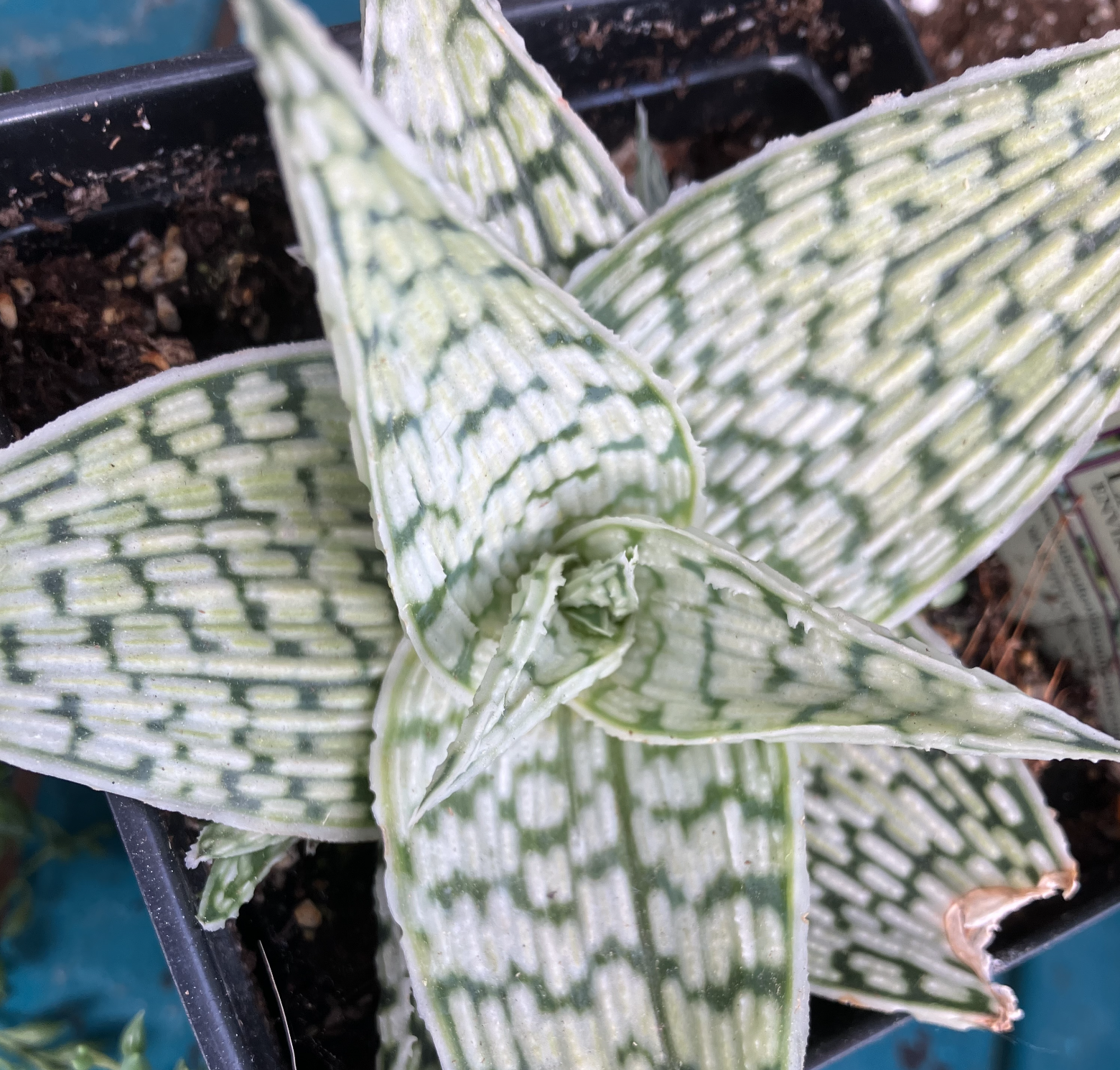Belousov-Zhabotinsky reaction¹	Giraffe fur pattern²	Haworthia leaf pattern

Pufferfish skin pattern³	Gasteria leaf pattern	Zebra fur pattern⁴

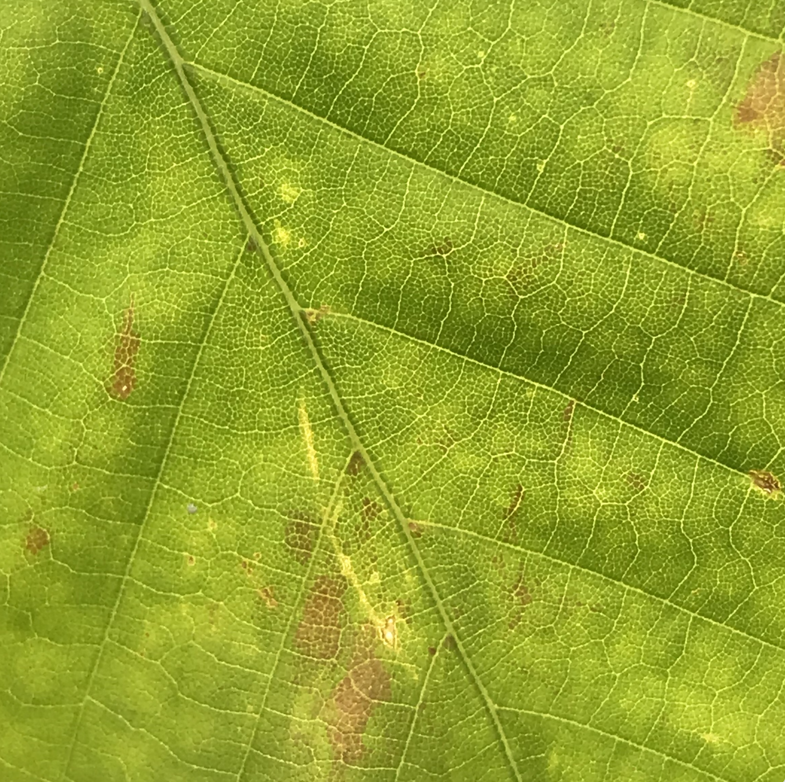Trout skin pattern	Lichen growth	Maple leaf veins

One first guess at how animal and plant patterns arise would be that they are hard-coded in deterministic genes. That would mean every limb, tooth, and stripe corresponds exactly to its specific description in a gene. However, the information storage requirements for this approach would be massive: every cell would have to have the entire blueprint for the entire organism, similar to why an uncompressed TIF file (where every pixel is described exactly) takes so much storage. An “uncompressed genome” describing an animal or plant would be immense, and such an organism’s fitness would likely collapse under the energetic and information-processing needs of such a genome.

So what if the genomes could have a “compressed genome” instead? Similar to a compressed tif file, where the images are essentially stored as partial instructions for how to reconstruct the images based on decompression rules (the decompression algorithm here is the other half of the reconstruction instructions). Here is where we have a more viable explanation of organismal patterning and development: encoding of rules for development (e.g. genes describing how to produce and react to a body landscape of diffusing morphogens).

Mathematician Alan Turing came up with a way to model this, which creates what is now known as a Turing Pattern.⁵ Through his paper called “The Chemical Basis of Morphogenesis”, he presents a mathematical system, called a “reaction-diffusion model” where two substances spread (diffuse) throughout the system interact with each other (react) and eventually a stable pattern emerges, which explains morphogenesis (the biological process that generates cell patterns and structures) A key feature of his explanation is that it uses simple, local rules to describe a way for these complex morphologies to arise. In fact, locality is a component of many physical systems we might be interested in modeling, a reflection of the physics of our universe.

Locality is also an important feature of cellular automata, where rule sets are given to all cells to automate the pattern formation in a model. This locality makes them effective for modeling a variety of physical processes such as pattern generation. The Gray-Scott model is a cellular automata that performs the reaction-diffusion computations and creates all the different Turing Patterns.

More recently, Neural Cellular Automatas (NCAs) have been created, including work by Niklasson et al. using NCA for textures⁶, published in distill. NCA models preserve the local dynamics of rule-based CA (and many physical systems besides), but use neural networks in place of rules based on logical or mathematical functions as in a conventional CA. Texture NCA can learn textures by iteratively updating the weights of its layers via the process of backpropagation to minimize the machine’s loss.

the loss in a machine learning model is a number that judges its performance as it is developing, with a lower score meaning a better performance. In a texture NCA, the loss judges how well the machine’s output matches the target texture. If you want to learn about how backpropagation works, this site explains it quite well.

What is exciting about NCAs model is that they may be able to learn plausible processes that could explain how different textural patterns are generated, including processes that might be further distilled into mathematical models like reaction-diffusion systems.

I worked with a similar implementation to Niklasson et al’s, called the Symbolic Regression Neural Cellular Automata (SRNCA) available here. Here is how the NCA gets a style loss for its texture:

First, the NCA model generates a texture by iteratively applying its neural layer operations to an image grid
Next, the final texture image is used as input to a pre-trained convolutional neural network layer (conv-net) (we used VGG16), which, in short, extracts features (such as vertical edges, horizontal edges, and points) using multiple layers of convolutions, and stores these features as vectors.
Next, a Gram matrix is calculated for several layers of the conv-net, which allows us to see how these vectors are correlated. A Gram matrix stores the dot product (the product of a vector with the other vector’s transpose, which measures how close they are) for every possible pair of vectors in each layer. We can write the value for the Gram matrix element at position (i,j) as

matmul_transpose

or as

dot_product

where the angle brackets and the dot are different ways of specifying the inner product. As a result, each Gram matrix has as many rows and columns as the number of channels in the layer.

At the same time as steps 2 and 3 for the training image, the target texture image (the image that the model is trying to make a similar pattern to) is also used directly as input to the conv-net model, and Gram matrices are calculated for the target image.
Finally, from the Gram Matrices from both the training image and the target texture image, the style loss is calculated: which is the mean squared error between the Gram matrices for the target image and the training image. This loss gives us a rating of the difference in textures, or style, (as parsed in the hidden layer features of the convolutional neural network) of an image rather than a direct pixel-by-pixel comparison. Again, the loss is used to update the NCA to repeat this entire process again and again to learn the texture.

You can visualize this process in this diagram:

Hyperparameter Exploration

I tested hyperparameters to learn more about their impact on the performance of the SRNCA, hoping to find insight into questions such as:

does any single hyperparameter affect the model output?
is there an optimal set of hyperparameters?
how are the hyperparameters related to each other and the model output?
does the same set of hyperparameters behave similarly across different training images?

The hyperparameters include:

Parameter	description
number of channels	grid channels (including RGB)
number of hidden channels	NCA hidden channels
max ca steps	maximum number of grid updates
batch size	number of samples in a batch
number of filters	number of (unlearned) perception kernels
update rate	proportion of pixels updated each ca step
learning rate	rate that modifies how quickly NCA parameters change

Perhaps the most obvious method for hyperparameter search (beyond manual adjustment by a human operator) is grid search: systematically looping through each set of possible values for each hyperparameter. Grid search is known to be inefficient at best, and random search represents an effective intermediate step between grid search and an additional optimization method over hyperparameters (e.g. an evolutionary algorithm). Random search over hyperparameters in general can be expected to give equal or better performance with a lower computational expense than grid search⁷.

So, the first thing I did was use random values for the hyperparameters with different target textures and see the result. I recorded the values for the parameters used, and the final loss that the algorithm gave, after 16383 steps.

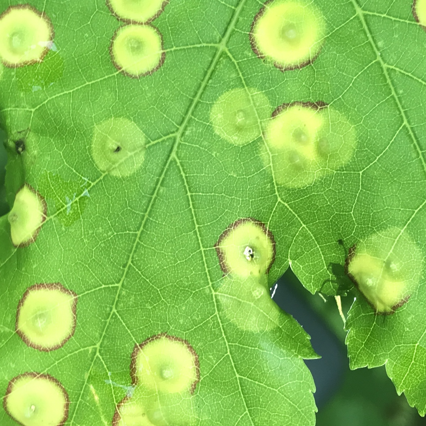
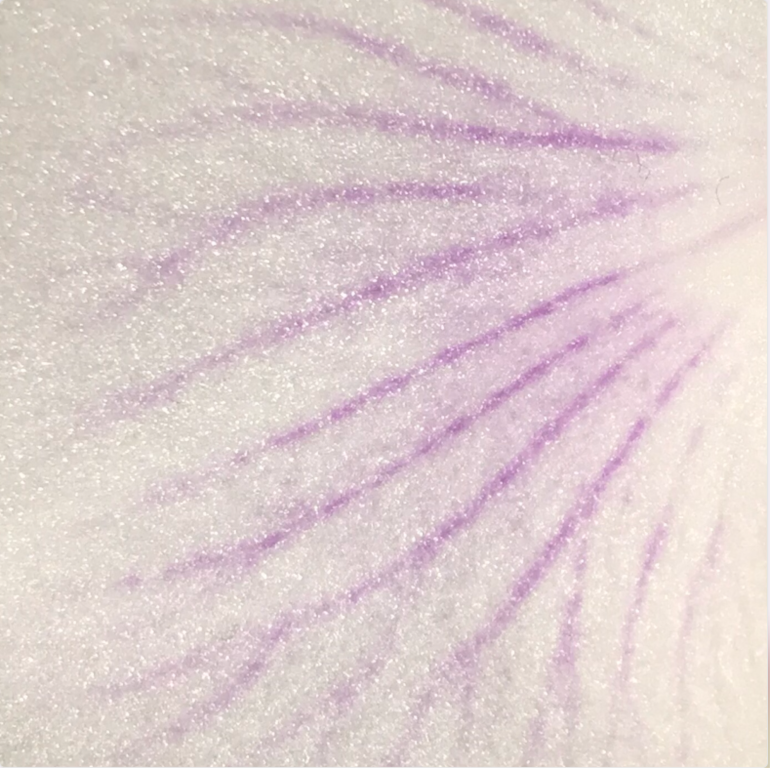
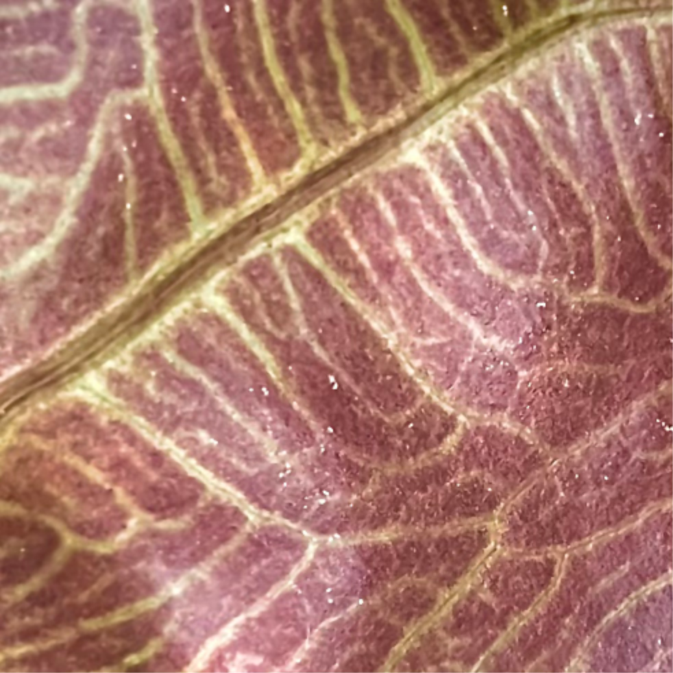
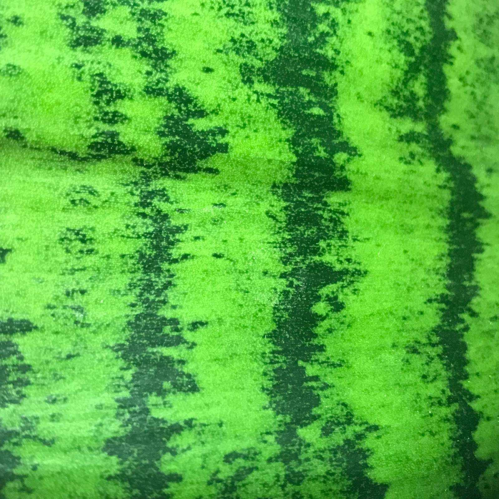
I was interested in creating plant textures with this algorithm, so the target textures I used were these four images of plants around my house, and gave them names that I’ll refer to throughout this post:

Roundleaf - Circular variegation from eggs laid on a maple leaf	Orchid Petal- Branching pigments on an orchid petal	Alocasia- Veins on the underside of an Alocasia leaf	Snake Plant- Striped variegation on a Snake Plant

I conducted most of my trials on the round leaf eggs texture leaf with eggs laid on it. What made this a great training image was that, out of these four textures, it had the highest variability in the final loss, the loss at step 16383. The loss usually ranged anywhere from .5 to 5. A higher variability of outcomes from the same parameters makes it easier to pinpoint specific trends because the data is more spread out.

Distribution of final losses across different textures in 10 different random sets of hyperparameters:

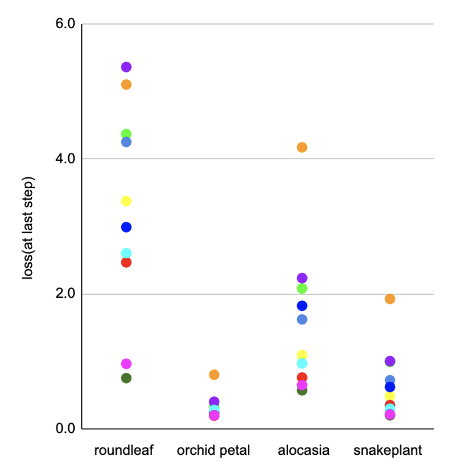Each set of hyperparameters was tested on each of the four textures and corresponds to a color. As shown, the roundleaf target image had the most variability.

Effectiveness of the Gram Function

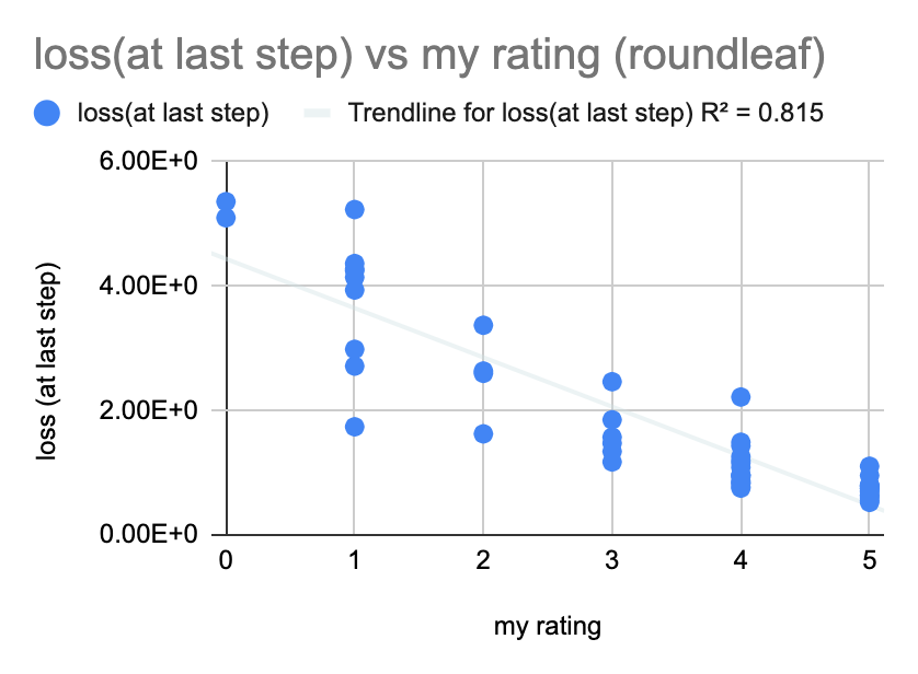
Firstly, apart from the hyperparameters themselves, I wanted to see how well the style loss (which if you remember from earlier, is calculated using Gram Matrices) judged the training image as it was developing. To do this, I simply plotted the final loss against my own rating of texture at its last step. I rated the textures on a scale of 0-5, with 5 being great: the color and unique patterns were extremely close to the target texture, and 0 being poor: the color or pattern was completely different from the target texture.

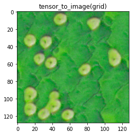
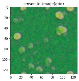
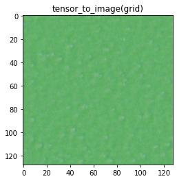
Here are some examples of generated textures and how I decided to score them: Target image: roundleaf eggs



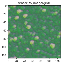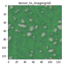
My rating: 5	My rating: 4	My rating: 3

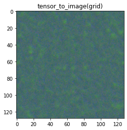My rating: 2	My rating: 1	My rating: 0

Looking at 50 random textures that were trained to reach the roundleaf eggs texture, there was a pretty strong negative linear relationship between the final loss and my rating, which makes sense as a lower loss should mean a better pattern. It shows that the Gram matrix is quite effective at capturing the elements of style important to at least one human viewer.

Relationships between parameter values and final output

There didn’t seem to be any convincing linear relationships, however, between the hyperparameters and the final loss, as shown by these graphs of parameter values versus the loss:

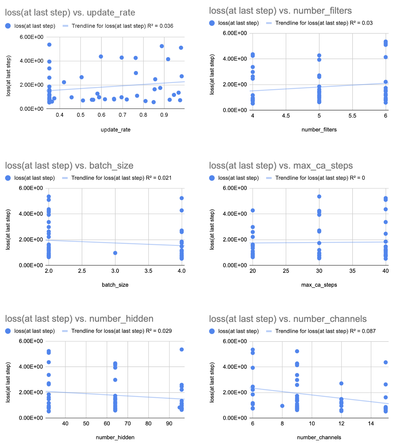
So, I looked at clusters to see if certain combinations of hyperparameters near certain values result in specific outcomes. I tried both the Principal Component Analysis⁸⁹ (PCA) model and the Uniform Manifold Approximation and Projection¹⁰ (UMAP) model. The Umap model always gave me unviable results to try, such as negative values for model channels, but I tried some of the suggestions that the PCA model gave me.

Although my sample size was only two, it seemed that the PCA model worked pretty well for finding a combination of parameters that generated a “good” pattern with a mean rating of 4.4:

From mean rating 4.4:

But, not so much for generating a “bad” pattern with a mean resting of .5. However, these textures do certainly appear to not be as great as the ones from the mean rating of 4.4:

From mean rating .5:

Noting that the PCA model is a linear model for dimensionality reduction and it yielded mediocre results, and that there were no notable correlations in linear fits to each individual hyperparameter as discussed earlier, it is likely that the parameters interact in a nonlinear way (for example, increasing the learning rate might only be better when you also increase the batch size). The UMAP model for gathering clusters of hyperparameters is non-linear, but it didn’t pass the sanity check of predicting hyperparameters I could actually use. A next step would be to try another nonlinear model, such as the Nonlinear PCA to uncover the ways the hyperparameters interact with each other to yield predictable results.

Performance relationships across different textures

Performance across different textures seemed to be the most tight relationship that I saw in exploring the hyperparameters. The way I tested this relationship was by generating 10 random sets of hyperparameters and testing them on all the four textures. I found that combinations that didn’t work well on one pattern didn’t do very well on the other textures, and combinations that did work well seemed to work great on others too.

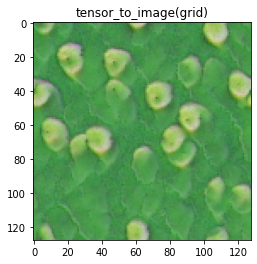
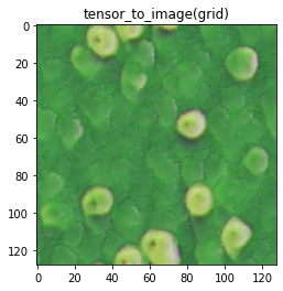
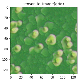
Hyperparameter set 5

For example, my fifth set yielded great results across the different target textures:

Parameter	number
channels	15
hidden channels	96
max ca steps	40
batch size	2
filters	4
update rate	0.559994317
learning rate	1e-05


	>
roundleaf	orchid petal

alocasia	snake plant

Hyperparameter set 8

And my eight set yielded horrible results across the different target textures:

Parameter	number
channels	6
hidden channels	32
max ca steps	40
batch size	2
filters	6
update rate	0.980292
learning rate	1e-05



roundleaf	orchid petal

alocasia	snake plant

At the end, I graphed the relationship between the roundleaf final loss versus other other textures’ final losses for each of the ten sets of parameters.

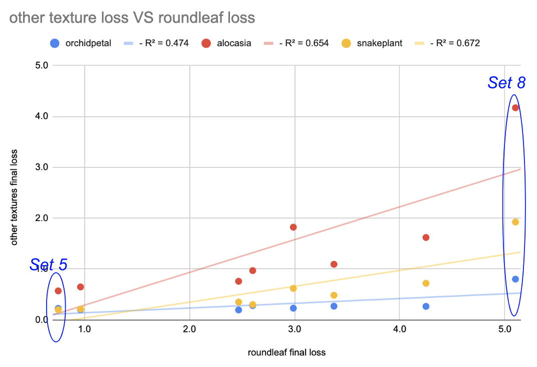
It showed a positive, linear correlation, meaning that as the set yielded a higher loss (a worse pattern) for the roundleaf texture, it would also yield a higher loss for the other textures, and vice versa. It was also interesting that each distribution had an increasing spread as the loss increased. This makes sense because as a set yields a less and less accurate result (increasing loss) for the roundleaf texture, there are more possibilities of textures to be generated which increases the range of possible outcomes for the other textures. Finally, even with only ten samples, each of the relationships seemed to have a y-intercept of approximately 0. This is notable because it suggests that a hyperparameter set that is extremely close to zero for one texture, would likely also minimize the loss for other textures too, and therefore that there is an optimal set of hyperparameters.

A next step for hyperparameter exploration in the algorithm is to find this optimal set by using an evolutionary strategy to evolve the parameters to the best combinations.

Conclusion

Project accomplishments

Trained NCA models to generate reasonable facsimiles of biologically generated patterns. The application of NCA texture models to plant morphogenesis ties the modern tools of automatic differentiation and neural networks back to Turing’s seminal work⁵, one of the founding works of mathematical biology.
Used random search to find reliable hyperparameters that work on multiple target image textures.
Explored using dimensionality reduction methods UMAP and PCA to generate good (and poor-performing) hyperparameters, but found these methods didn’t fully capture the effect of hyperparameters (or predicted non-viable hyperparameters). If you would like to see these results yourself, or play around with these models and the data, you can use this notebook I used
Combined with poor linear fits of individual hyperparameters to style loss, the observation that small perturbations in principal components about a high-performing P.C cluster suggests that the interaction between hyperparameters is likely synergistic and nonlinear, and could be better captured with a nonlinear model.

Ideas for future work

Using nonlinear PCA (neural network autoencoders) to capture nonlinear interactions between and generate effective combinations of hyperparameters.
Using evolution strategies to augment random search by updating hyperparameters distributions over multiple generations to find an optimal set of hyperparameters

It was nice to see first-hand how well the SRNCA model can learn textures, even from pictures of random plants around my house. If you would like to do some hyperparameter exploration on this model yourself, you can use this notebook that I used.

Sources

Tim Kench. (2011). The Belousov-Zhabotinsky Oscillating Reaction. Youtube. Retrieved August 26, 2022, from https://www.youtube.com/watch?v=PpyKSRo8Iec. ↩
Sutter, B. (2022). Close-up of Giraffe Body Skin Fur. Pexels.com. Retrieved September 2, 2022, from https://www.pexels.com/photo/close-up-of-giraffe-body-skin-fur-12406721/. ↩
Dato-on, A. (n.d.). Yellow and Black Pufferfish Swimming in the Aquarium. pexels.com. Retrieved August 26, 2022, from https://www.pexels.com/photo/yellow-and-black-pufferfish-swimming-in-the-aquarium-9408366/. ↩
Anonymous. (2017). Zebra Fur. Pexels.com. Retrieved September 2, 2022, from https://www.pexels.com/photo/zebra-fur-70376/. ↩
Turing, A. (1970, January 1). [PDF] the chemical basis of morphogenesis: Semantic scholar. undefined. Retrieved August 26, 2022, from https://www.semanticscholar.org/paper/The-chemical-basis-of-morphogenesis-Turing/d635e2843c6fb034e9126aa73ef9c2e4e2c4714d ↩ ↩²
Niklasson, E., Mordvintsev, A., Randazzo, E., & Levin, M. (2021, May 7). Self-organising textures. Distill. Retrieved August 26, 2022, from https://distill.pub/selforg/2021/textures/ ↩
Bergstra, J., & Bengio, Y. (1970, January 1). [PDF] random search for hyper-parameter optimization: Semantic scholar. undefined. Retrieved August 26, 2022, from https://www.semanticscholar.org/paper/Random-Search-for-Hyper-Parameter-Optimization-Bergstra-Bengio/188e247506ad992b8bc62d6c74789e89891a984f ↩
Karl Pearson F.R.S. (1901) LIII. On lines and planes of closest fit to systems of points in space, The London, Edinburgh, and Dublin Philosophical Magazine and Journal of Science, 2:11, 559-572, DOI: 10.1080/14786440109462720 ↩
Hotelling, H. (1933). Analysis of a complex of statistical variables into principal components. Journal of Educational Psychology, 24, 417–441, and 498–520. ↩
McInnes, L., & Healy, J. (1970, January 1). [PDF] UMAP: Uniform Manifold approximation and projection for dimension reduction: Semantic scholar. undefined. Retrieved August 26, 2022, from https://www.semanticscholar.org/paper/UMAP%3A-Uniform-Manifold-Approximation-and-Projection-McInnes-Healy/3a288c63576fc385910cb5bc44eaea75b442e62e ↩